Computing functional diversity indices and community weighted means for fishes. • fwtraits

The fwtraits access the www.freshwaterecology.info database that contains several ecological parameters, traits, and indicators used in biogeographical modeling, functional diversity and taxonomic assessments, and environmental monitoring. These are grouped based on the taxonomic groups, including macroinvertebrates, fishes, phytoplankton, phytobenthos, and macrophytes. Therefore, in this workflow, we demonstrated using ecological parameters from the database in assessing functional diversity.

library(fwtraits)
library(ggplot2)

Fishes data used in the analysis

We tested using the species data with both spatial coordinates to auto-generate sites or sites already indicated in the sites or species data.

data("speciesdata")

set.seed(1135)
speciesdata$abund <- rnorm(n = nrow(speciesdata), 4.3, 1.2)

#species with geographical coordinates

geospdata <- speciesdata |> 
  sf::st_as_sf(coords = c('decimalLongitude', 'decimalLatitude'), 
               crs = sf::st_crs(4326))

Retrieving the ecological parameters from the database

We considered two ecological references for fishes: rheophily habitat, spawning habitat, and feeding diet adult. These were selected because most species have records, reducing missing values that might have required imputation.

It should be noted that imputing for missing traits is outside the scope of this package. So, species that do not have records were dropped when computing the functional diversity indices or community weighted means.


fishtraits <- fw_fetchdata(data = speciesdata, 
                         ecoparams = c('rheophily habitat', 'spawning habitat',
                                       'feeding diet adult'), 
                         taxonomic_column = 'scientificName',
                         organismgroup = 'fi')

1. Compute functional diversity indices

These are computed by setting FD to TRUE and abund parameter must be provided. They the indices are computed using the FD package (Laliberté & Legendre 2010). The indices tested included Functional richness (FRic), species richness (SRic), Functional evenness (FEve), Functional diversity (FDiv), Functional dispersion (FDis), and Rao quotient (Rao Q).


#fd indices calculated when abundance  is provided.

fdindices <- fw_fdcompute(fwdata = fishtraits, 
                        sitesdata = speciesdata,
                        sites = 'waterBody',
                        species = 'scientificName',
                        abund = 'abund',
                        FD = TRUE)
head(fdindices, 3)
#>     site      FRic SRic      FEve      FDiv     FDis      RaoQ
#> 1  Colne 0.7837022   14 0.6666667 0.7514879 3.130064 10.274519
#> 2 Mersey 0.9073171   16 0.7142857 0.7992736 3.148708 10.713105
#> 3 Thames 0.7852545   14 0.5471074 0.7493893 2.843325  8.656933

#functional richness only: when abundance is not provided.
fdric<- fw_fdcompute(fwdata = fishtraits, 
                        sitesdata = speciesdata,
                        sites = 'waterBody',
                        species = 'scientificName',
                        FD = TRUE)
head(fdric, 3)
#>         site      FRic SRic
#> 1        Usk 0.5381900    6
#> 2       Taff 0.1459965    3
#> 3 River Lune 0.3203472    3

2. Compute Functional Diversity indices using autogenerated sites.


#fd indices calculated when abundance  is provided.

geofdind <- fw_fdcompute(fwdata = fishtraits, 
                        sitesdata = geospdata,
                        species = 'scientificName',
                        abund = 'abund',
                        FD = TRUE)
head(geofdind, 3)
#>    site      FRic SRic      FEve      FDiv     FDis      RaoQ
#> 1 99116 0.7837022   14 0.6658334 0.7486573 3.146454 10.355734
#> 2 99172 0.7828410   12 0.6645772 0.7600437 2.927213  9.374808
#> 3 99260 0.7852545   12 0.6256742 0.7396812 2.880293  8.890285

#functional richness only: when abundance is not provided.
geofd <- fw_fdcompute(fwdata = fishtraits, 
                        sitesdata = geospdata,
                        species = 'scientificName',
                        FD = TRUE)
head(geofd, 3)
#>   site      FRic SRic
#> 1  991        NA    2
#> 2  993        NA    1
#> 3  994 0.1459965    3

3. Visualisation of the ecological paramter for each index.


df <- fdindices |> tidyr::gather('fdind', "vals", -site)
                                 
ggplot(data = df, aes(site, vals, fill = fdind))+
  geom_bar(stat = 'identity')+
  scale_fill_viridis_d()+
  theme(legend.position = "none",
        axis.text.x = element_text(angle = 45, hjust = 1, size = 7))+
  facet_wrap(~fdind, scales ='free_y')+
  scale_y_continuous(expand = expansion(mult = c(0, 0.1)))+
  labs(x='sites', y='FD indices')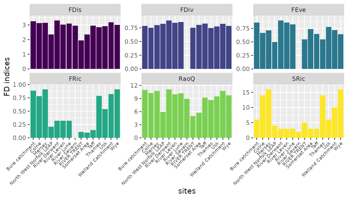


#Functional richness

dffric <- fdric |> tidyr::gather('fdind', "vals", -site)
                                 
ggplot(data = dffric, aes(site, vals, fill = fdind))+
  geom_bar(stat = 'identity')+
  scale_fill_viridis_d()+
  theme(legend.position = "none",
        axis.text.x = element_text(angle = 45, hjust = 1, size = 7))+
  facet_wrap(~fdind, scales ='free_y')+
  scale_y_continuous(expand = expansion(mult = c(0, 0.1)))+
  labs(x='Sites', y='FD indices')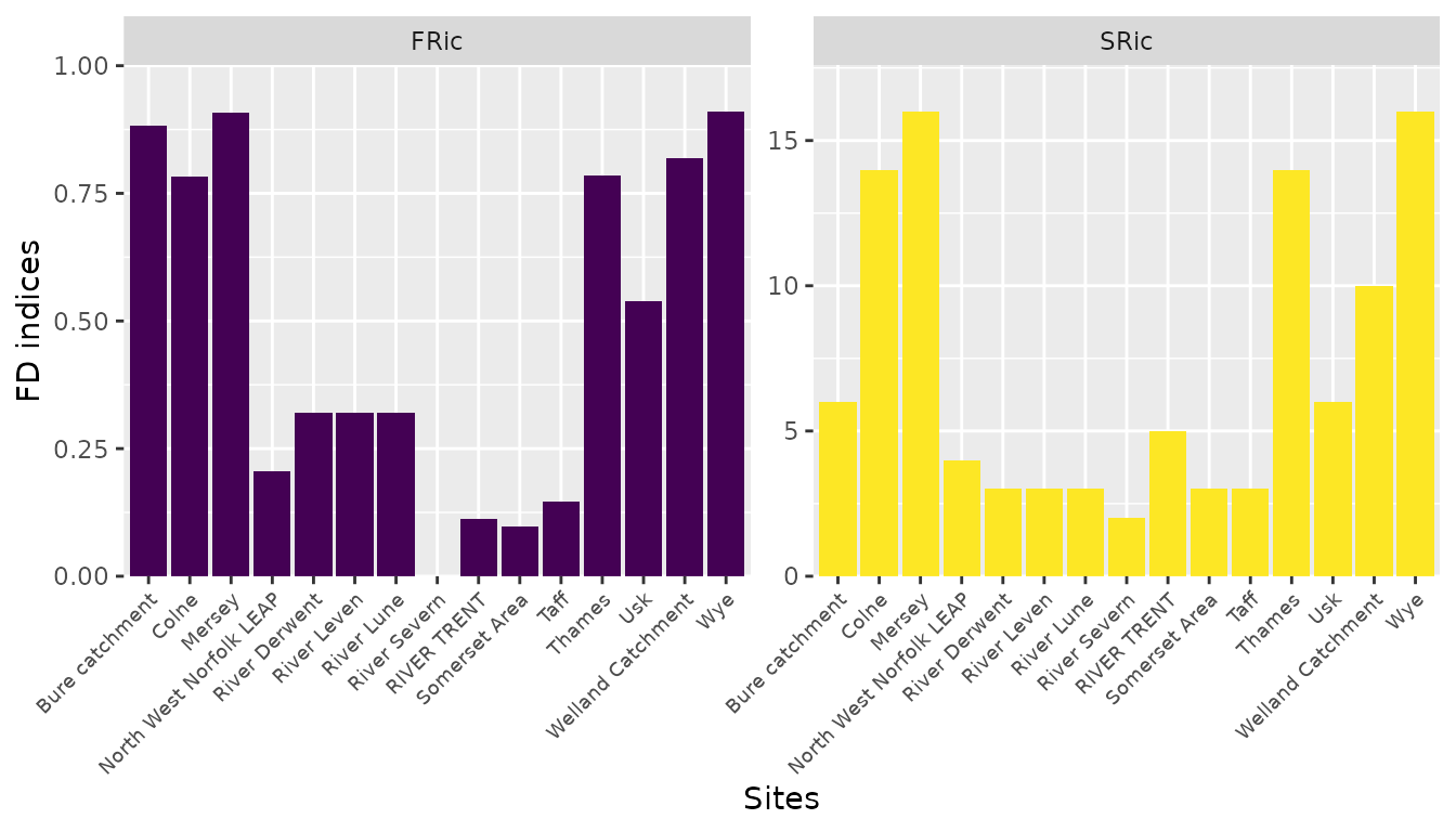

4. Compute community weighted means.

Community weighted means measures how traits vary with environmental change (Guy-Haim & Bouchet 2025).

cwmdata <- fw_fdcompute(fwdata = fishtraits, 
                        sitesdata = speciesdata,
                        sites = 'waterBody',
                        species = 'scientificName',
                        abund = 'abund',
                        FD = FALSE)
head(cwmdata, 3)
#>     site X.rheophily.habitat.eurytopic X.rheophily.habitat.limnophilic
#> 1  Colne                     0.4598488                      0.12751814
#> 2 Mersey                     0.3665371                      0.05518399
#> 3 Thames                     0.4602653                      0.03823995
#>   X.rheophily.habitat.rheophilic X.rheophily.habitat.rheophilic.A
#> 1                              0                        0.3424712
#> 2                              0                        0.5095482
#> 3                              0                        0.4475848
#>   X.rheophily.habitat.rheophilic.B X.spawning.habitat.euryoparous
#> 1                       0.07016187                      0.4440039
#> 2                       0.06873071                      0.2894240
#> 3                       0.05390994                      0.2242217
#>   X.spawning.habitat.limnoparous X.spawning.habitat.rheoparous
#> 1                      0.2029570                     0.3530391
#> 2                      0.2081951                     0.5023809
#> 3                      0.2596240                     0.5161543
#>   X.feeding.diet.adult.detritivorous X.feeding.diet.adult.invertivorous
#> 1                         0.00000000                          0.3449768
#> 2                         0.06693826                          0.3845350
#> 3                         0.00000000                          0.2437924
#>   X.feeding.diet.adult.omnivorous X.feeding.diet.adult.piscivorous
#> 1                       0.5043557                        0.1506675
#> 2                       0.4272511                        0.1212756
#> 3                       0.6405770                        0.1156306

5. Compute community weighted means using raw traits.

In this approach, this does not require fuzzy coding of the trait data. This is necessary for community weighted means.

cwmdata2 <- fw_fdcompute(fwdata = fishtraits, 
                        sitesdata = speciesdata,
                        sites = 'waterBody',
                        species = 'scientificName',
                        abund = 'abund',
                        FD = FALSE, dummy = FALSE)
head(cwmdata2, 3)
#>     site rheophily.habitat_eurytopic rheophily.habitat_limnophilic
#> 1  Colne                   0.4598488                    0.12751814
#> 2 Mersey                   0.3665371                    0.05518399
#> 3 Thames                   0.4602653                    0.03823995
#>   rheophily.habitat_rheophilic rheophily.habitat_rheophilic.A
#> 1                            0                      0.3424712
#> 2                            0                      0.5095482
#> 3                            0                      0.4475848
#>   rheophily.habitat_rheophilic.B spawning.habitat_euryoparous
#> 1                     0.07016187                    0.4440039
#> 2                     0.06873071                    0.2894240
#> 3                     0.05390994                    0.2242217
#>   spawning.habitat_limnoparous spawning.habitat_rheoparous
#> 1                    0.2029570                   0.3530391
#> 2                    0.2081951                   0.5023809
#> 3                    0.2596240                   0.5161543
#>   feeding.diet.adult_detritivorous feeding.diet.adult_invertivorous
#> 1                       0.00000000                        0.3449768
#> 2                       0.06693826                        0.3845350
#> 3                       0.00000000                        0.2437924
#>   feeding.diet.adult_omnivorous feeding.diet.adult_piscivorous
#> 1                     0.5043557                      0.1506675
#> 2                     0.4272511                      0.1212756
#> 3                     0.6405770                      0.1156306

Refereences

Laliberté, E., & Legendre, P. (2010). A distance‐based framework for measuring functional diversity from multiple traits. Ecology, 91(1), 299-305.
Guy-Haim, T., & Bouchet, V. M. (2025). Beyond taxonomy: A framework for biological trait analysis to assess the functional structure of benthic foraminiferal communities. Marine Pollution Bulletin, 213, 117699.