Flag outliers based on species ecological ranges. • specleanr

library(specleanr)

Introduction to outlier detection based on species ecological ranges.

Species ecological ranges provide the ecological limits within which the species can survive or reproduce within the ecosystem. These ranges are usually obtained from experimental setups or continued data collection. However, the species’ ecological ranges may vary due to colonization of new ranges. Therefore, if the species ecological ranges are available, then records obtained outside the ranges can be flagged as outliers that require further analysis.
The sources of species ecological ranges include standard databases such as FishBase (Froese and Pauly 2014), www.freshwaterecology.info (Schmidt-Kloiber and Hering 2015), or the International Union for Conservation of Nature. Linking to these databases is not outside the scope of this package. Still, a user can collate a table of species’ ecological ranges and use it in this package’s multidetect function to flag outliers.
This method of using species ecological ranges is concertedly used with the other outlier detection methods, including univariate and multivariate methods, as shown below.

Example using species ecological ranges with other outlier detection methods.

1 Loading example datasets

data("jdsdata")
data("efidata")

wcd <- terra::rast(system.file('extdata/worldclim.tiff', package = "specleanr"))

#match and clean

matchd <- match_datasets(datasets = list(jds= jdsdata, efi =efidata),
                         lats = 'lat', lons = 'lon',
                         country = 'JDS4_site_ID',
                         species = c('scientificName', 'speciesname'),
                         date=c('sampling_date','Date'))

#matchclean <- check_names(matchd, colsp = 'species', verbose = FALSE, merge = TRUE)

db <- sf::read_sf(system.file('extdata/danube.shp.zip',
                              package = "specleanr"), quiet = TRUE)

2. Extracting environmental predictors from worldclim dataset


refdata <- pred_extract(data = matchd, raster = wcd,
                        lat = 'decimalLatitude',
                        lon = 'decimalLongitude',
                        bbox = db,
                        colsp = 'species',
                        list = TRUE,
                        verbose = FALSE,
                        minpts = 6,
                        merge = FALSE)

3. Preparing ecological ranges for Squalius cephalus

NOTE

The species ecological ranges are made for explanatory purposes, but do not reflect the species ecological ranges.
optdata includes five columns, including 1) species, which indicates the species names being studied. The names should be the same as those in the reference dataset. 2) mintemp is the minimum temperature of the species (lower ecological limit). 3) maxtemp is the species’ maximum temperature (upper ecological limit). 4) meantemp is the species mean temperature, and 5) direction, which signifies whether it is greater or lower than in the case of the mean temperature.


sqcep <- refdata["Squalius cephalus"]

optdata <- data.frame(species= c("Squalius cephalus", "Abramis brama"),
                      mintemp = c(6, 1.6),maxtemp = c(8.588, 21),
                      meantemp = c(8.5, 10.4), #ecoparam
                      direction = c('greater', 'greater'))

4. Outlier detection with univariate, multivariate and species ecological ranges

The multiple parameter is set to TRUE even when one species is considered because the data is extracted from refdata dataset that has multiple species.
The optpar is provided in a list format and since the mintemp and maxtemp are provided, then the dirction of whether greater or lower are not required to be set.


squalius_outlier <- multidetect(data = sqcep, multiple = TRUE,
                      var = 'bio1',
                      output = 'outlier',
                      exclude = c('x','y'),
                      methods = c('zscore', 'adjbox', 'optimal', 'kmeans', "logboxplot", "hampel"),
                      optpar = list(optdf=optdata, optspcol = 'species',
                                    mincol = "mintemp", maxcol = "maxtemp"))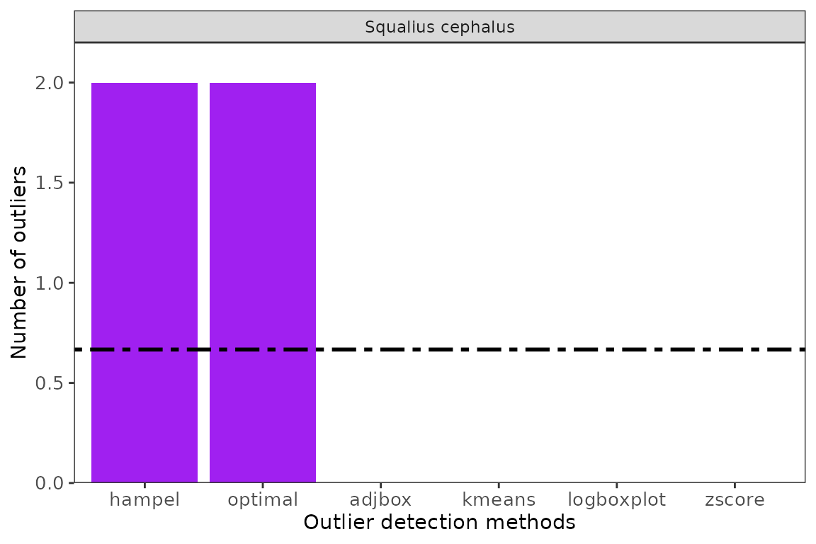

Visualise the number of outliers detected by each method


ggoutliers(squalius_outlier)

Obtaining quality controlled dataset using loess method or data labeling


squalius_qc_loess <- extract_clean_data(refdata = sqcep, 
                                      outliers = squalius_outlier, loess = TRUE)

#clean dataset
nrow(squalius_qc_loess)
#> [1] 19

#reference data
nrow(sqcep[[1]])
#> [1] 19

squalius_qc_labeled <- classify_data(refdata = sqcep, outliers = squalius_outlier)

Visualise labelled quality controlled dataset



ggenvironmentalspace(squalius_qc_labeled, 
                     type = '1D',
                     ggxangle = 45, 
                     scalecolor = 'viridis',
                     xhjust = 1,
                     legend_position = 'blank',
                     ylab = "Number of records",
                     xlab = "Outlier labels")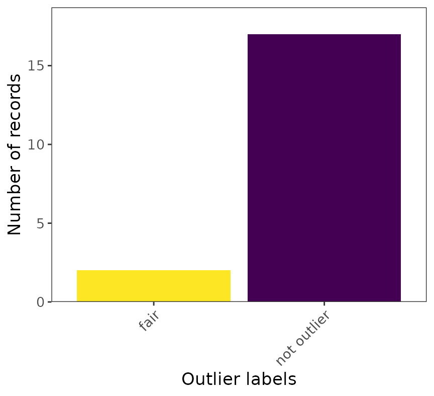

Summary explanation

Outliers were flagged by species optimal ranges and the Hampel method; however, these were not flagged in other methods, which meant that these were not substantially absolute outliers. Consequently, based on outlier classification, only fair and not outlier ctageories were observed.

References

Schmidt-Kloiber, A., & Hering, D. (2015). www. freshwaterecology. info–an online tool that unifies, standardizes and codifies more than 20,000 European freshwater organisms and their ecological preferences. Ecological Indicators, 53, 271-282.
Froese. R and Pauly D (2014). FishBase. world wide web electronic publication. fishbase. org.