Environmental outlier detection with bootstrapping and principal component analysis.
Source:vignettes/eOutlier.Rmd
eOutlier.RmdEnvironmental outlier check for fish species from the Danube River Basin
The workflow for environmental outlier detection and removal is
similar across taxa, regions, or ecological realms. However, we included
the check_names() function to cater for
fish species names exhaustively. In this worked example, we tested the
functionalities on the fish species from the Danube River Basin, with
extracts of species records from Joint Danube Survey (JDS) and EFI+ data
archived in the package. We complimented the data with fish species
occurrences from online sources including Global Biodiversity
Information Facility (GBIF), iNaturalist, and VertNET using the
getdata() function. They are basically
five steps, including: 1) Data acquisition and harmonization; 2)
Precleaning and predictor extraction 3) outlier detection 4)
identification of clean data and suitable method 5) developing species
distribution models (optional).
Scope of application
In this workflow, we provide three approaches that can be used to handle outlier detection, namely 1) the default approach (no bootstrapping and principal component analysis applied); 2) bootstrapping applied during outlier detection mostly for fewer records (user based to set the records) and 3) combining principal component analysis and bootstrapping. Because each approach will significantly affect how records are flagged as outliers, its upon the user to select an approach to use. However, we advise users to apply bootstrapping and PCA if the particular suspicious records are still not handled in the first approach.
1.Data acquisition: a) Collate species species records: offline and online data
The species records were obtained from the archived datasets
extracted from the Joint Danube Survey (https://www.danubesurvey.org/jds4/) and EFIPLUS (Logez
et al., 2012). To compliment species records, we used the
getdata() function to retrieve data from
the GBIF (https://www.gbif.org/), VertNet (http://www.vertnet.org/)
and iNaturalist ( https://www.inaturalist.org/) for Squalius
cephalus, Salmo trutta, Thymallus thymallus, and
Anguilla anguilla. For online data, we limited data to 50
records from each data source to reduce on the execution time.
NOTE
This workflow may fail if the particular settings such as blocking of IP address to GIBF, iNaturalist, FishBase, and VertNet may prevent user from accessing the online data. Since, this may differ at user-to-user basis, it is beyond the scope of this package to address such limitations.
#==========================
#Step 1ai. Obtain Local data sources (archived in this package)
#=========================

data(efidata) #Data extract from EFIPLUS data

data(jdsdata) #Data extract from JDS4 data

#===================================
#Step 1aii: Retrieve online datas for the species: polygon to limit the extent to get records.
#=====================================
danube <- sf::st_read(system.file('extdata', "danube.shp.zip",
                                  package = 'specleanr'), quiet=TRUE)

# df_online <- getdata(data = c("Squalius cephalus", 'Salmo trutta',
#                               "Thymallus thymallus","Anguilla anguilla"),
#                                 extent = danube,
#                                 gbiflim = 50,
#                                 inatlim = 50,
#                                 vertlim = 50,
#                      verbose = FALSE)
data(fishdata)

dim(fishdata)
#> [1] 400   8
Merging and harmonizing species records from different sources
The online data sources from getdata()
and local files are merged using the
match_datasets() function. Five columns
are harmonized while combining data from different sources: the country,
species names, latitude/longitude columns, and dates. The Darwin Core
standard names are country, species, decimalLatitude, decimalLongitude,
and dates (Wieczorek et al., 2012). So, if the local dataset has a
different name for standard names, the user should indicate it. For
example, in JDS data, the species column is labeled
speciesname, shown in the species parameter for
automatic renaming and merging with other datasets. * Note: The user
should indicate all dataset names in the list. *
check_names() is used to clean species names in terms of
synonyms or spellings, based on FishBase (https://www.fishbase.se/). This function generates
another column speciescheck that contain the clean
names.
mergealldfs <- match_datasets(datasets = list(efi= efidata, jds = jdsdata,
                                        fishdata = fishdata),
                country = c('JDS4_sampling_ID'),
                lats = 'lat', lons = 'lon',
                species = c('speciesname', 'scientificName'))

#Species names are re-cleaned since the species names from vertnet are changed.

cleannames_df <- check_names(data = mergealldfs, colsp = 'species', pct = 90,
                             merge = TRUE, verbose = TRUE)
#> The synoynm Salmo trutta fario will be replaced with Salmo trutta.
#> The synoynm Salmo trutta lacustris will be replaced with Salmo trutta.
#> The synoynm Aspius aspius will be replaced with Leuciscus aspius.

#Filter out species from clean names df where the species names such as synonyms like Salmo trutta fario chnaged to Slamo trutta

speciesfiltered <- cleannames_df[cleannames_df$speciescheck %in%
                                   c("Squalius cephalus", 'Salmo trutta',
                                     "Thymallus thymallus","Anguilla anguilla"),]
1. Data acquisition: b) Environmental predictors from worldclim
We used WORLDCLIM data archived in the package to enable users to
test the package functions seamlessly. For direct interaction with the
WORDCLIM data, please visit (https://www.worldclim.org/) and the
geodata package for download in
user-customized workflows. WORLDCLIM data has 19 bioclimatic variables
(https://www.worldclim.org/data/bioclim.html),
including;
-
BIO1= Annual Mean Temperature -
BIO2= Mean Diurnal Range (Mean of monthly (max temp - min temp)) -
BIO3= Isothermality (BIO2/BIO7) (×100) -
BIO4= Temperature Seasonality (standard deviation ×100) -
BIO5= Max Temperature of Warmest Month -
BIO6= Min Temperature of Coldest Month -
BIO7= Temperature Annual Range (BIO5-BIO6) -
BIO8= Mean Temperature of Wettest Quarter -
BIO9= Mean Temperature of Driest Quarter -
BIO10= Mean Temperature of Warmest Quarter -
BIO11= Mean Temperature of Coldest Quarter -
BIO12= Annual Precipitation -
BIO13= Precipitation of Wettest Month -
BIO14= Precipitation of Driest Month -
BIO15= Precipitation Seasonality (Coefficient of Variation) -
BIO16= Precipitation of Wettest Quarter -
BIO17= Precipitation of Driest Quarter -
BIO18= Precipitation of Warmest Quarter -
BIO19= Precipitation of Coldest Quarter
#Get climatic variables from the package folder

worldclim <- terra::rast(system.file('extdata/worldclim.tiff', package = 'specleanr'))
2. Precleaning and environmental data extraction
Here,
The duplicate records are removed if points they are obtained from the same location for the same species.
The missing values coordinates are removed.
The environmental predictors are extracted from the raster layers (WORLDCLIM).
The user can set the minimum point for the species to be retianed for further analyis.
The bounding box can be set to limit the extent of data extraction. For this case, we used the basin layer for the Danube Basin was obtained from Hydrography90m (https://hydrography.org/hydrography90m/hydrography90m_layers).
The user can either return a dataframe or list of the cleaned data. Important in the next steps.
#Get basin shapefile to delineate the study region: optional

danube <- sf::st_read(system.file('extdata', 'danube.shp.zip',
                                  package = 'specleanr'), quiet=TRUE)

#For multiple species indicate multiple TRUE
multipreclened <-  pred_extract(data= speciesfiltered,
                             raster= worldclim,
                             lat = 'decimalLatitude',
                             lon = 'decimalLongitude',
                             colsp = 'speciescheck',
                             bbox  = danube,
                             list= TRUE,
                             minpts = 10, merge = FALSE)
names(multipreclened)
#> [1] "Anguilla anguilla"   "Salmo trutta"        "Squalius cephalus"
#> [4] "Thymallus thymallus"


thymallusdata <- speciesfiltered[speciesfiltered[,'speciescheck'] %in%c("Thymallus thymallus"),]

dim(thymallusdata)
#> [1] 130   7

thymallus_referencedata <-  pred_extract(data= thymallusdata, raster= worldclim,
                             lat = 'decimalLatitude',
                             lon = 'decimalLongitude',
                             colsp = 'speciescheck',
                             bbox  = danube,
                             list= TRUE,
                             minpts = 10)
dim(thymallus_referencedata)
#> [1] 82 21
3. Outlier detection for both single and multiple species (No PCA or bootstrapping)
Multiple outlier detection are set. This package contains 20 outlier
detection methods and the user can run
extractMethods() to get the allowed
methods. They are categorized into univariate, multivariate and species
ecological ranges. * var is the predictor to be used
univariate methods. * exclude allows to remove predictors
that user deems unnecessary. For example, the coordinates, since the
multivariate methods consider the whole dataset.
#For multiple species: default settings

multiple_spp_out_detection <- multidetect(data = multipreclened,
                      multiple = TRUE,
                      var = 'bio6',
                     exclude = c('x','y'),
                      methods = c('zscore', 'adjbox',
                                                'logboxplot', 'distboxplot',
                                                'iqr', 'semiqr',
                                                'hampel','kmeans',
                                                'jknife', 'onesvm',
                                                'iforest'))
#single species:default settings

thymallus_outlier_detection <- multidetect(data = thymallus_referencedata,
                      multiple = FALSE,
                      var = 'bio6',
                      output = 'outlier',
                      exclude = c('x','y'),
                      methods = c('zscore', 'adjbox',
                                  'logboxplot', 'distboxplot',
                                  'iqr', 'semiqr',
                                  'hampel','kmeans',
                                  'jknife', 'onesvm',
                                  'iforest'))
4. Outlier visualization for single and multiple species
-
ggoutliersare based in ggplot2, so it can be modified based on user needs. x: is the output for outlier detection, y is the species name or index for multiple species, and raw = TRUE if the number of outliers are the displayed, otherwise the proportion of outliers to the total number of records will be plotted.
#for multiple species
ggoutliers(multiple_spp_out_detection)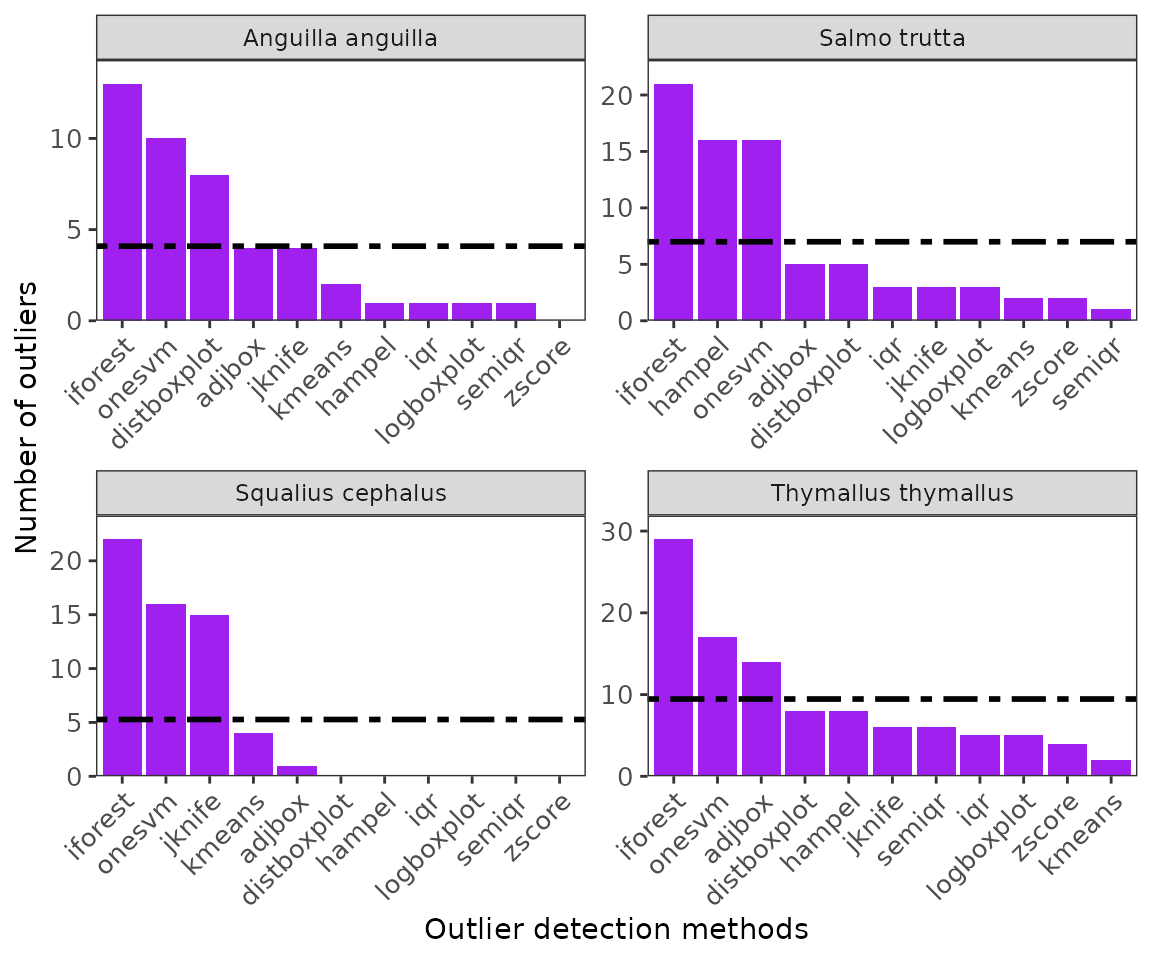
#for single species
ggoutliers(thymallus_outlier_detection)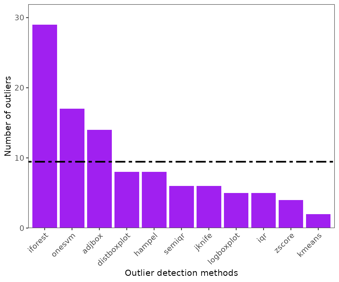
Identify the best threshold using loess model.
The local regression is used to optimize and identify the best threshold for denoting the point as an absolute outlier. We fit the local region model between the data retained at every threshold, and we identify a maxima when the number of records retain are number of records retained does not significantly vary with an increased increase in the threshold.
thymallus_opt_threshold <- optimal_threshold(refdata = thymallus_referencedata,
                               outliers = thymallus_outlier_detection, plot = list(plot = TRUE, group = "Thymallus thymallus"))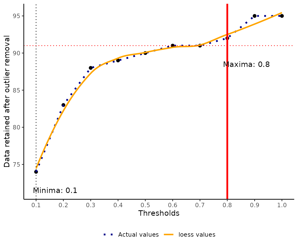
#obtain the optimal thresholds for multiple species

multspp_opt_threshold <- optimal_threshold(refdata = multipreclened,
                                           outliers = multiple_spp_out_detection)
5. Extracting clean data from the reference data (precleaned data in step 2).
The user sets a threshold ranging from 0.1 to 1 but its advisable to set a value above 0.5 to include above 50% of the methods. threshold is the value indicating the proportion of methods to be used to classify a record as a true outlier. For example, a threshold of 0.6 means that at least in the 4 of the 6 methods noted during outlier detection in step 3. We used the loess method for identifying the optimal threshold.
multspecies_clean <- extract_clean_data(refdata = multipreclened,
                                        outliers = multiple_spp_out_detection,
                                        loess =  TRUE)
head(multspecies_clean)
#>       bio1     bio2     bio3     bio4     bio5     bio6     bio7     bio8
#> 1 8.340094 8.558521 31.95564 691.9463 23.15800 -3.62450 26.78250 15.38925
#> 2 7.765240 8.342354 31.78373 687.5156 21.74550 -4.50175 26.24725 16.19358
#> 3 7.765240 8.342354 31.78373 687.5156 21.74550 -4.50175 26.24725 16.19358
#> 4 7.765240 8.342354 31.78373 687.5156 21.74550 -4.50175 26.24725 16.19358
#> 5 8.390240 8.568895 31.32536 722.0088 23.12525 -4.22925 27.35450 17.21496
#> 6 6.954260 7.829604 29.42382 723.2756 21.54375 -5.06600 26.60975 15.78113
#>         bio9    bio10       bio11 bio12 bio13 bio14    bio15 bio16 bio17 bio18
#> 1  1.1871250 16.93192 -0.08562502   789    97    44 28.08648   274   136   274
#> 2  0.6048333 16.19358 -0.60591668  1364   175    79 25.91408   479   270   479
#> 3  0.6048333 16.19358 -0.60591668  1364   175    79 25.91408   479   270   479
#> 4  0.6048333 16.19358 -0.60591668  1364   175    79 25.91408   479   270   479
#> 5  0.9156250 17.21496 -0.48479167  1142   143    68 23.92640   391   228   391
#> 6 -0.7299168 15.78113 -1.92591667   608    91    29 41.44856   244    90   244
#>   bio19        x        y            groups
#> 1   145 10.08333 48.41667 Anguilla anguilla
#> 2   274 13.58333 47.91667 Anguilla anguilla
#> 3   274 13.58333 47.91667 Anguilla anguilla
#> 4   274 13.58333 47.91667 Anguilla anguilla
#> 5   230 13.75000 48.08333 Anguilla anguilla
#> 6    97 16.75000 49.41667 Anguilla anguilla

thymallus_qcdata <- extract_clean_data(refdata = thymallus_referencedata,
                             outliers = thymallus_outlier_detection,
                             loess = TRUE)


multiple_spp_qcdata <- classify_data(refdata = multipreclened,
                                outliers = multiple_spp_out_detection,
                                EIF = TRUE)
head(multiple_spp_qcdata)
#>       bio1     bio2     bio3     bio4     bio5     bio6     bio7     bio8
#> 2 7.765240 8.342354 31.78373 687.5156 21.74550 -4.50175 26.24725 16.19358
#> 3 7.765240 8.342354 31.78373 687.5156 21.74550 -4.50175 26.24725 16.19358
#> 4 7.765240 8.342354 31.78373 687.5156 21.74550 -4.50175 26.24725 16.19358
#> 5 8.390240 8.568895 31.32536 722.0088 23.12525 -4.22925 27.35450 17.21496
#> 7 9.624270 8.874875 30.36663 766.5389 25.47275 -3.75300 29.22575 18.99033
#> 8 8.464437 8.629666 32.26737 690.2155 22.73925 -4.00500 26.74425 16.96646
#>        bio9    bio10       bio11 bio12 bio13 bio14    bio15 bio16 bio17 bio18
#> 2 0.6048333 16.19358 -0.60591668  1364   175    79 25.91408   479   270   479
#> 3 0.6048333 16.19358 -0.60591668  1364   175    79 25.91408   479   270   479
#> 4 0.6048333 16.19358 -0.60591668  1364   175    79 25.91408   479   270   479
#> 5 0.9156250 17.21496 -0.48479167  1142   143    68 23.92640   391   228   391
#> 7 1.6068749 18.99033  0.13245833   690    85    37 29.31466   245   117   245
#> 8 1.2360415 16.96646  0.07987499  1143   146    64 30.75084   422   207   422
#>   bio19        x        y       label            groups         EIF
#> 2   274 13.58333 47.91667 not outlier Anguilla anguilla -0.24635227
#> 3   274 13.58333 47.91667 not outlier Anguilla anguilla -0.24635227
#> 4   274 13.58333 47.91667 not outlier Anguilla anguilla -0.24635227
#> 5   230 13.75000 48.08333 not outlier Anguilla anguilla  0.03853413
#> 7   126 17.25000 48.25000 not outlier Anguilla anguilla  0.53643179
#> 8   207 12.41667 47.91667 not outlier Anguilla anguilla  0.27297715


thymallus_qc_labelled <- classify_data(refdata = thymallus_referencedata,
                              outliers = thymallus_outlier_detection,
                              EIF = TRUE)
head(thymallus_qc_labelled)
#>       bio1     bio2     bio3     bio4     bio5     bio6     bio7     bio8
#> 1 8.464437 8.629666 32.26737 690.2155 22.73925 -4.00500 26.74425 16.96646
#> 3 8.130990 9.155687 33.54192 693.5986 22.50525 -4.79100 27.29625 16.58138
#> 4 8.091240 8.933604 32.88585 694.5287 22.77500 -4.39050 27.16550 16.61037
#> 5 7.765240 8.342354 31.78373 687.5156 21.74550 -4.50175 26.24725 16.19358
#> 6 8.130990 9.155687 33.54192 693.5986 22.50525 -4.79100 27.29625 16.58138
#> 7 7.519135 8.307521 31.21427 699.6627 21.70950 -4.90500 26.61450 16.09933
#>        bio9    bio10       bio11 bio12 bio13 bio14    bio15 bio16 bio17 bio18
#> 1 1.2360415 16.96646  0.07987499  1143   146    64 30.75084   422   207   422
#> 3 0.9313333 16.58138 -0.41912505  1307   174    69 33.66177   499   233   499
#> 4 0.8317083 16.61037 -0.43866670   808   106    42 32.08204   296   135   296
#> 5 0.6048333 16.19358 -0.60591668  1364   175    79 25.91408   479   270   479
#> 6 0.9313333 16.58138 -0.41912505  1307   174    69 33.66177   499   233   499
#> 7 0.2436249 16.09933 -1.03108346  1213   158    69 26.63618   427   238   427
#>   bio19        x        y       label       EIF
#> 1   207 12.41667 47.91667 not outlier 1.5813610
#> 3   234 13.08333 47.75000 not outlier 0.7856575
#> 4   138 11.75000 48.41667 not outlier 1.1911018
#> 5   274 13.58333 47.91667 not outlier 1.0784784
#> 6   234 13.08333 47.75000 not outlier 0.7856575
#> 7   239 13.91667 47.91667 not outlier 0.6702498
6. Visualize labeled data in environmental space.
#multiple species
ggenvironmentalspace(qcdata = multiple_spp_qcdata,
                     xvar = 'bio1',
                     yvar = "bio18",
                     xlab = "Annual mean temperature",
                     ylab = "Precipitation of Warmest Quarter",
                     scalecolor = 'viridis',
                     ncol = 2,
                     nrow = 2,
                     pointsize = 2)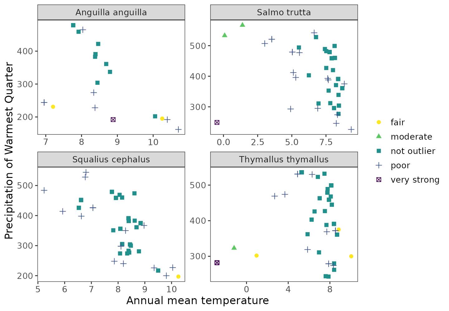
#for single species
ggenvironmentalspace(qcdata = thymallus_qc_labelled,
                     xvar = 'bio1',
                     yvar = "bio18",
                     xlab = "Annual mean temperature",
                     ylab = "Precipitation of Warmest Quarter",
                     scalecolor = 'viridis',
                     pointsize = 2)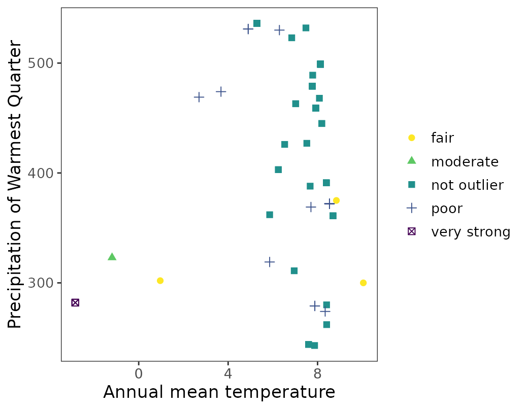
Using bootstrapping during outlier detection
Bootstrapping is a robust approach where the records are randomly sampled with replacement. In this approach, outlier detection is iteratively conducted on bootstrap samples and each record flagged as outlier is weighted based on the total number of bootstraps used. The higher the record is flagged in several across multiple tests, the higher the likelihood of record being an absolute outlier. Although the default number of records at bootstrapping is 30, the maximum number of records can be adjusted by the user as demonstrated below.
Note
Bootstrapping is not implemented by the defualt, so the user has to set it run during outlier detection.
The number of records maxrecords in reference dataset for Thymallus thymallus is 99. Therefore, to implement bootstrapping, indicate the maximum number of records higher than the nrows in reference dataset otherwise bootstrap will not be implemented.
The number of bootstraps, nb are user-defined.
Bootstrapping was conducted on Thymallus thymallus data because there was no proper separation between the moderate and very strong outliers.
thymallus_outlier_boot <- multidetect(data = thymallus_referencedata,
                      multiple = FALSE,
                      var = 'bio6',
                      exclude = c('x','y'),
                      methods = c('zscore', 'adjbox',
                                  'logboxplot', 'distboxplot',
                                  'iqr', 'semiqr',
                                  'hampel','kmeans',
                                  'jknife', 'onesvm',
                                  'iforest'),
                      bootSettings = list(run = TRUE, maxrecords = 100, nb = 10))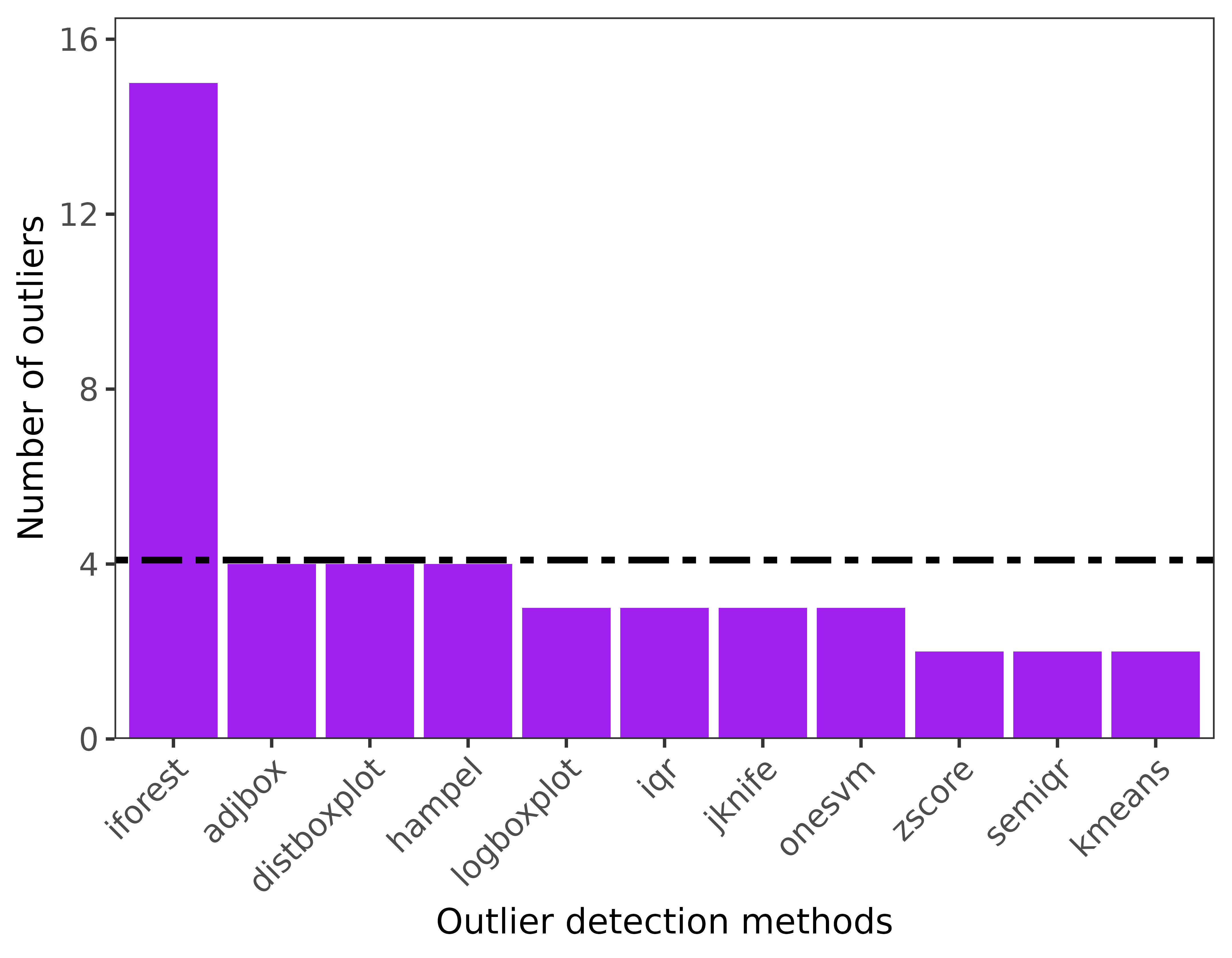
Classify data to obtain labels
thymallus_qc_label_boot <- classify_data(refdata = thymallus_referencedata,
                                outliers = thymallus_outlier_boot)
Visualise after bootstrapping
ggenvironmentalspace(qcdata = thymallus_qc_label_boot,
                     xvar = 'bio1',
                     yvar = "bio18",
                     xlab = "Annual mean temperature",
                     ylab = "Precipitation of Warmest Quarter",
                     scalecolor = 'viridis',
                     pointsize = 2)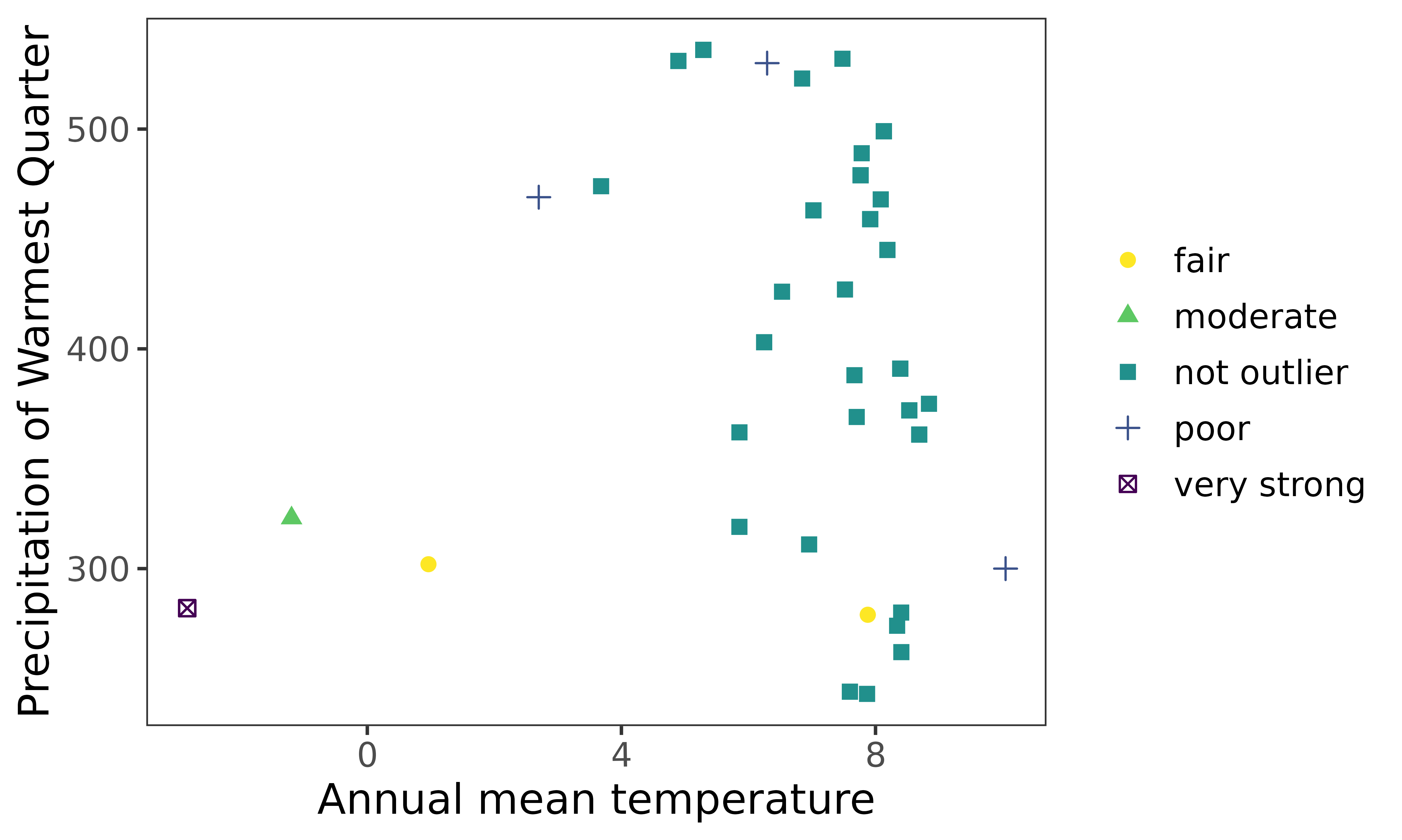
Note
When bootstrapping is applied, the very strong outlier turned into moderate outlier.
Apply principal component analysis and bootstrapping on Thymallus thymallus data.
Principal component analyis is a dimension reduction approach vital for highly multidimensional datasets. The user can decide to apply either PCA and bootstrapping or only one of them.
The number of principal components to be returned are changed using npc argument.
The visualise the cummulation variance captured in the principal components, the argument q is used.
thymallus_outlier_boot_pca <- multidetect(data = thymallus_referencedata,
                      multiple = FALSE,
                      var = 'bio6',
                      exclude = c('x','y'),
                      methods = c('zscore', 'adjbox',
                                  'logboxplot', 'distboxplot',
                                  'iqr', 'semiqr',
                                  'hampel','kmeans',
                                  'jknife', 'onesvm',
                                  'iforest'),
                      bootSettings = list(run = TRUE, maxrecords = 100, nb = 10),
                      pc = list(exec = TRUE, npc = 6, q = FALSE))
#> The cummulative proprotion for PCs 6 is 0.99173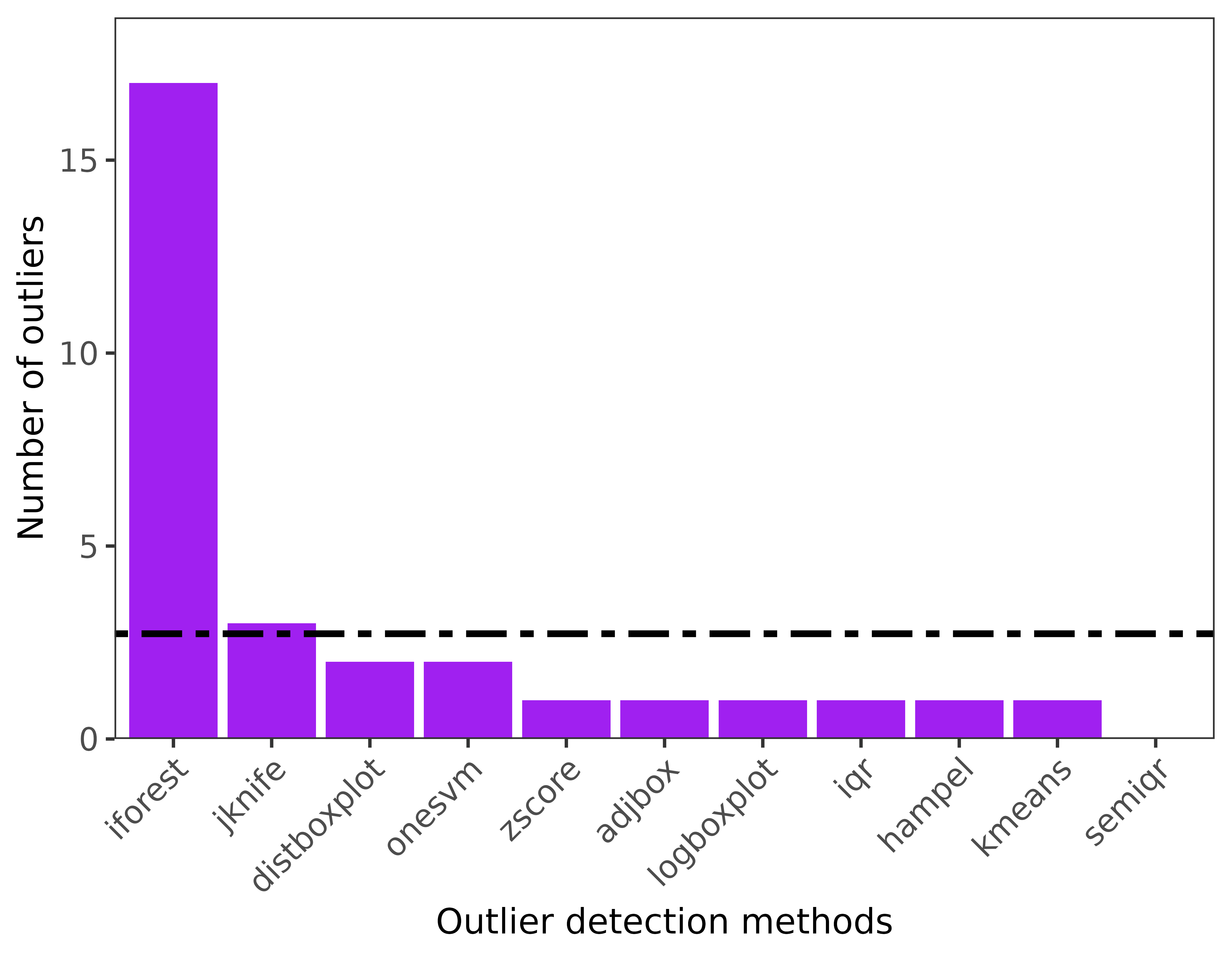
Classify data to obtain labels
thymallus_qc_label_boot_pca <- classify_data(refdata = thymallus_referencedata,
                                outliers = thymallus_outlier_boot_pca)
Visualise after bootstrapping
ggenvironmentalspace(qcdata = thymallus_qc_label_boot_pca,
                     xvar = 'bio1',
                     yvar = "bio18",
                     xlab = "Annual mean temperature",
                     ylab = "Precipitation of Warmest Quarter",
                     scalecolor = 'viridis',
                     pointsize = 2)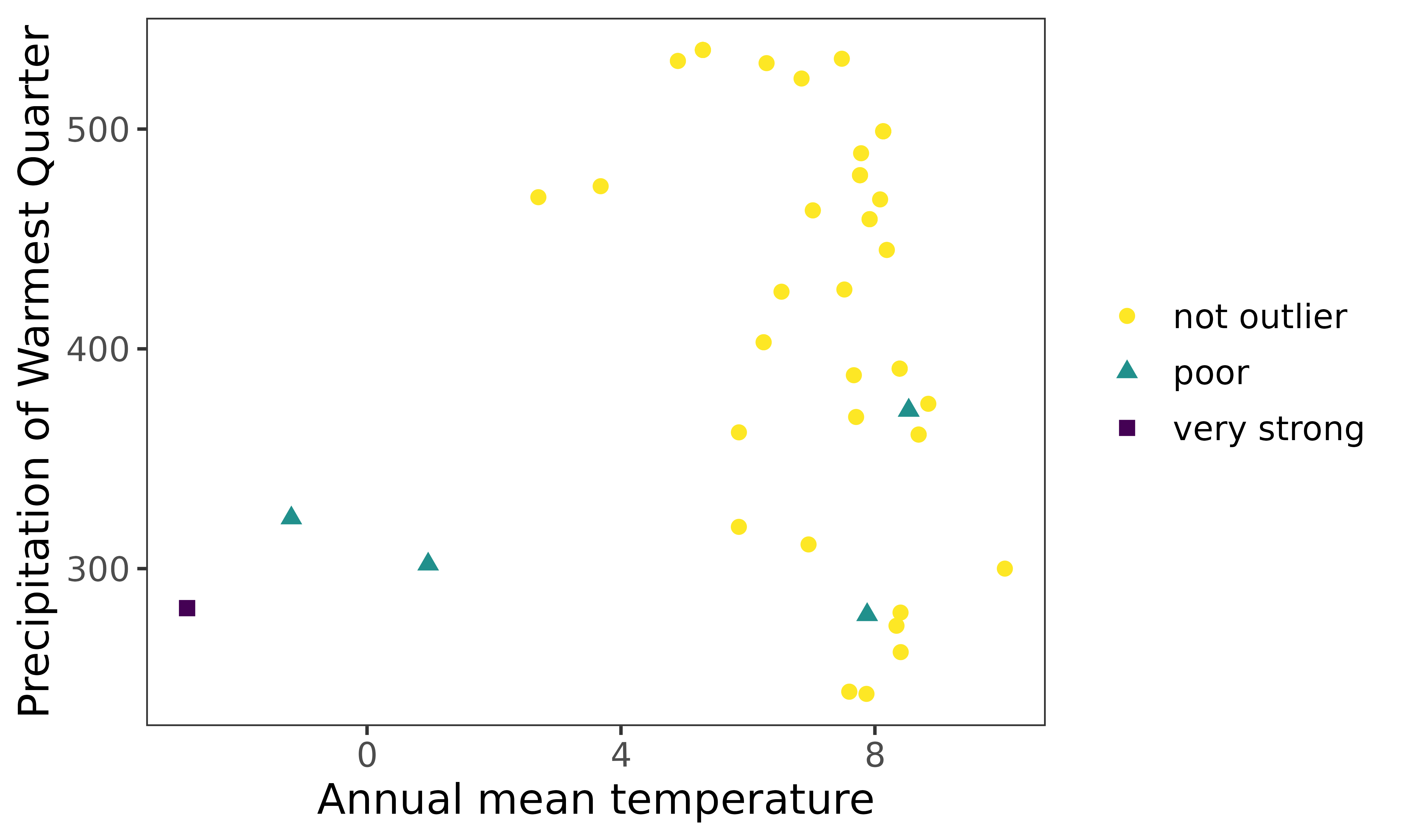
Notes
Coupling PCA and bootstrapping are robust approaches to handle outlier detection. In this example, moderate outlier turned into poor outliers.
References
- Wieczorek, J., Bloom, D., Guralnick, R., Blum, S., Döring, M., Giovanni, R., Robertson, T., & Vieglais, D. (2012). Darwin core: An evolving community-developed biodiversity data standard. PLoS ONE, 7(1). https://doi.org/10.1371/journal.pone.0029715