Detecting environmental outliers in species distribution models for plants. • specleanr


library(specleanr)

Detect environmental outliers for species occurrences in Fagus sylvatica, and Populus nigra* records based on bioclimatic data*.

To test the workflow on two plant species, namely the black poplar (Populus nigra) , which is a pioneer wind-pollinated deciduous tree from the Salicaceae family (de Rigo et al., 2016). The tree is distributed across Europe, Asia, and northern Africa (de Rigo et al., 2016; Harvey-Brown et al., 2017) and predominantly in flood plains in mixed forests (Harvey-Brown et al., 2017). The mature tree lives up to 300 to 400 years (de Rigo et al., 2016), and it has been assessed as data deficient according to IUCN RedList (Harvey-Brown et al., 2017). Secondly, we considered the European beech or common beech (Fagus sylvatica), which is also a deciduous hardy tree species that can tolerate various soil habitats but is not tolerant of waterlogged areas (Barstow et al., 2018). Although mature individuals have declined, the tree species IUCN RedList threat status is assessed as Least Concern (Barstow et al., 2018).

1. Data acquisition: a) species records

Data was retrieved from the iNaturalist (https://www.inaturalist.org/) and Global Biodiversity Information Facility-GBIF (https://www.gbif.org/). We use the getdata() function, built around rvertnet, rgbif, and rinat packages. We limited the occurrence records from GBIF to 700 and iNaturalist to 100. * Note: If the user has locally saved data, then after extracting the online data, the match_datasets() function can be used to merge all the data sets.

We set the bounding box (extent) parameter for getdata() to return only records within the Danube basin. However, the user can set this to suit the area of concern. If not set, the user data will download records globally, which is time-consuming and likely to break during the download. Therefore, it is strongly advisable to set the bounding box. Also, if a shapefile is available, the user can provide it instead of the bounding box, and the function will automatically extract the bounding box.


plantdf <- getdata(data = c( "Populus nigra", "Fagus sylvatica"), 
                    gbiflim = 700, inatlim = 100,
                     hasCoordinate = TRUE, 
                   extent = list(xmin = 8.15250, ymin = 42.08333, xmax=29.73583, ymax = 50.24500),
                   verbose = FALSE, warn = FALSE)

1. Data acquisition: b) Environmental predictors

We used WORLDCLIM data archived in the package to enable users to test the package functions seamlessly. For direct interaction with the WORDCLIM data, please visit (https://www.worldclim.org/) and the geodata package for download in user-customized workflows. WORLDCLIM data has 19 bioclimatic variables (https://www.worldclim.org/data/bioclim.html) (Amatulli et al., 2022), including

BIO1 = Annual Mean Temperature
BIO2 = Mean Diurnal Range (Mean of monthly (max temp - min temp))
BIO3 = Isothermality (BIO2/BIO7) (×100)
BIO4 = Temperature Seasonality (standard deviation ×100)
BIO5 = Max Temperature of Warmest Month
BIO6 = Min Temperature of Coldest Month
BIO7 = Temperature Annual Range (BIO5-BIO6)
BIO8 = Mean Temperature of Wettest Quarter
BIO9 = Mean Temperature of Driest Quarter
BIO10 = Mean Temperature of Warmest Quarter
BIO11 = Mean Temperature of Coldest Quarter
BIO12 = Annual Precipitation
BIO13 = Precipitation of Wettest Month
BIO14 = Precipitation of Driest Month
BIO15 = Precipitation Seasonality (Coefficient of Variation)
BIO16 = Precipitation of Wettest Quarter
BIO17 = Precipitation of Driest Quarter
BIO18 = Precipitation of Warmest Quarter
BIO19 = Precipitation of Coldest Quarter


#Get climatic variables from the package folder

worldclim <- system.file('extdata/worldclim.tiff', package = 'specleanr')

worldclim <- terra::rast(worldclim)

2. Preliminary analysis

The step involves removing missing coordinate values, setting the geographical range for the data collated in 1.a, if the user did not set the bounding box during data download. After that, the environmental data predictors are extracted. The user can set either parameter list = TRUE to return a list of datasets for each species, if multiple species are considered, or list = FALSE to return a combined dataframe. The Danube basin was collated from the Hydrography90m basin files (https://hydrography.org/hydrography90m/hydrography90m_layers).


danube_basin <- sf::st_read(system.file('extdata', "danube.shp.zip", package = 'specleanr'), 
                            quiet = TRUE)

#Environmental predictors extraction for multiple species (multiple = TRUE)

multspreference_data <-  pred_extract(data= plantdf, 
                             raster= worldclim, 
                             lat = 'decimalLatitude',
                             lon = 'decimalLongitude',
                             colsp = 'species',  
                             bbox = danube_basin,
                             list= TRUE, 
                             minpts = 10, merge = FALSE, verbose = FALSE, warn = FALSE)

#Environmental prediction extraction for a single species (multiple = FALSE)
fagus_data_filtered <- subset(plantdf, species=="Fagus sylvatica")

fagus_data_reference <-  pred_extract(data= fagus_data_filtered, 
                             raster= worldclim, 
                             lat = 'decimalLatitude',
                             lon = 'decimalLongitude',
                             colsp = 'species',  
                             bbox = danube_basin, 
                             minpts = 10, merge = FALSE, 
                           verbose = FALSE, warn = FALSE)

3. Detecting outliers using multiple outlier detection methods

To detect outliers we selected ensembled seven outlier detection methods at least from different categories i.e., 1) univariate methods: adjusted boxplot adjbox(), Hampel filter: hampel(), Z-score zscore() and reverse jackknifing jknife(); 2) Multivariate methods or machine learning models: local outlier factor: lof(), K-means: kmeans(), and Mahalanobis distance measure mahal().


#Flag outlier in single species data (multiple = TRUE)
multspp_outliers <- multidetect(data = multspreference_data,
                       multiple = TRUE,
                       var = 'bio1',
                       output = 'outlier',
                       exclude = c('x','y'), 
                       methods = c('adjbox', "hampel", 'zscore', 
                                   'lof', 'jknife', 'kmeans', 'mahal'),
                       silence_true_errors = FALSE, warn = F, verbose = F)

#Flag outlier in single species data (multiple = FALSE)

fagus_outliers <- multidetect(data = fagus_data_reference,
                       multiple = FALSE,
                       var = 'bio1',
                       output = 'outlier',
                       exclude = c('x','y'), 
                       methods = c('adjbox', "hampel", 'zscore', 
                                   'lof', 'jknife', 'kmeans', 'mahal'),
                       silence_true_errors = FALSE, warn = F, verbose = F)

Visualizing outliers flagged by each method

The plots are wrapped on a ggplot2 object and extensible with ggplot2 parameters. The ggoultiers() takes in 3 parameters: 1: x the outlier object of datacleaner class; 2: y the index or species name if the outlier has more than one species, and 3: raw to either indicate the number of outlier if TRUE or proportional or outliers flagged about total number of occurrences if FALSE


ggoutliers(x=multspp_outliers)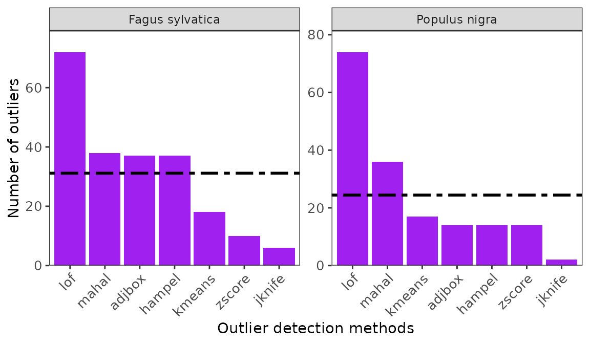


#for one species: no index needed
ggoutliers(x= fagus_outliers)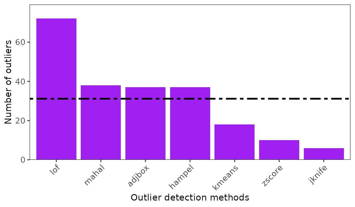

### Identify the best threshold using loess model.


optimal1<- optimal_threshold(refdata = fagus_data_reference, outliers = fagus_outliers, plot = TRUE)



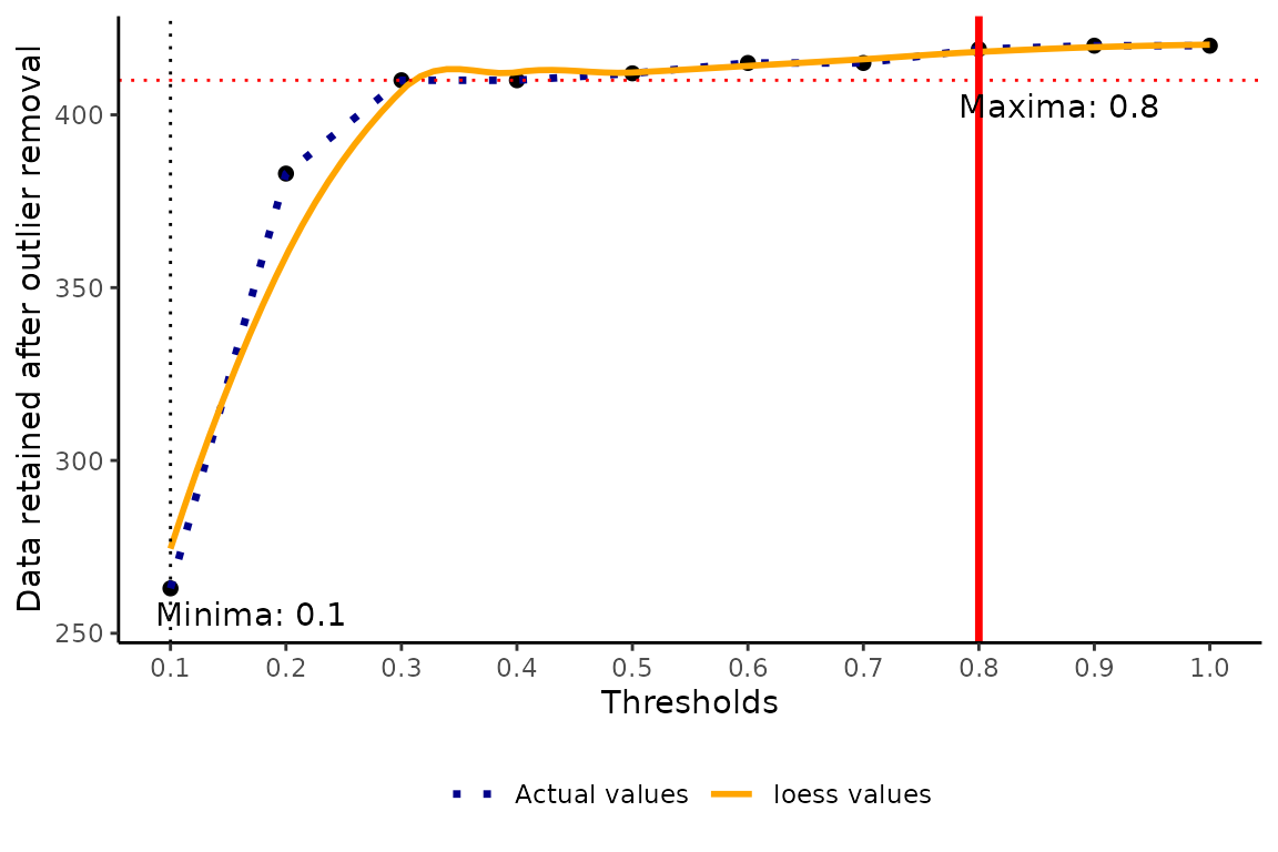
optimalthreshold <- optimal_threshold(refdata = multspreference_data, outliers = multspp_outliers, plot = FALSE)

4. Extracting clean data set after outlier detection

The mode can be set to mode = abs to discard only absolute outliers or mode = best to use the best method. The outlier flagged by the best method will be used to clean the data. For more information, check (Basooma et al., 2025).


multspp_qc_data <- extract_clean_data(refdata = multspreference_data, 
                                      outliers = multspp_outliers,
                                      loess = TRUE)

multspp_qc_label <- classify_data(refdata = multspreference_data, 
                                      outliers = multspp_outliers)


fagus_qc_data <- extract_clean_data(refdata = fagus_data_reference, 
                                    outliers = fagus_outliers,
                                    loess = TRUE)

fagus_qc_label <- classify_data(refdata = fagus_data_reference, 
                                    outliers = fagus_outliers)

Visualising records in environmental space


#for single species
ggenvironmentalspace(qcdata = fagus_qc_label,
                     xvar = 'bio1',
                     yvar = "bio18",
                     xlab = "Annual mean temperature",
                     ylab = "Precipitation of Warmest Quarter",
                     scalecolor = 'viridis',
                     pointsize = 2)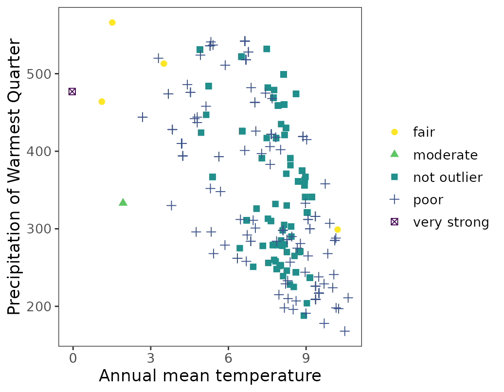


#for single species
ggenvironmentalspace(qcdata = multspp_qc_label,
                     xvar = 'bio1',
                     yvar = "bio18",
                     xlab = "Annual mean temperature",
                     ylab = "Precipitation of Warmest Quarter",
                     scalecolor = 'viridis',
                     pointsize = 2)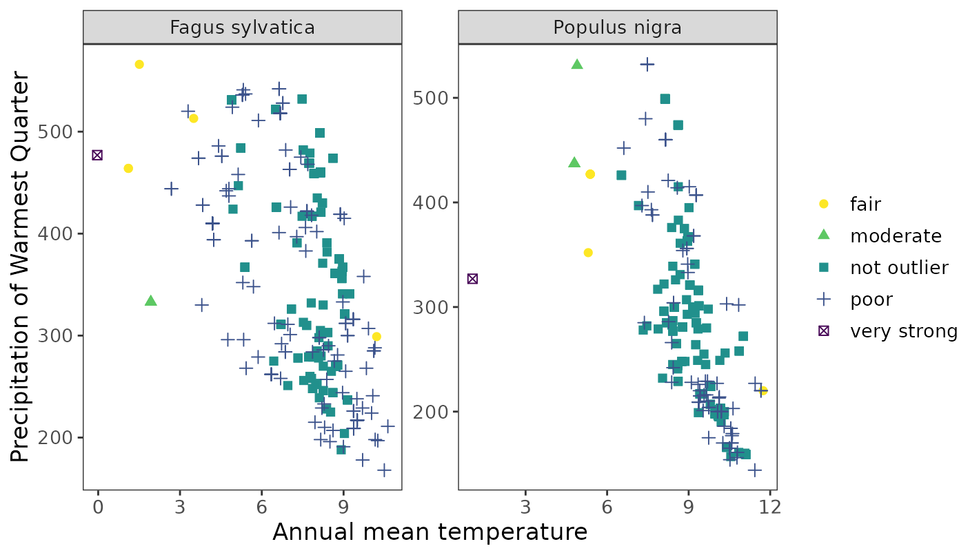

Visualising records in environmental space in 3d


#for single species
ggenvironmentalspace(qcdata = fagus_qc_label,
                     xvar = 'bio1',
                     yvar = "bio18",
                     zvar = 'bio6',
                     type = "3d",
                     labelvar = "label",
                     xlab = "Annual mean temperature",
                     ylab = "Precipitation of Warmest Quarter",
                     zlab = "Min Temperature of Coldest Month",
                     scalecolor = 'viridis',
                     lpos3d = "right",
                     pointsize = 2)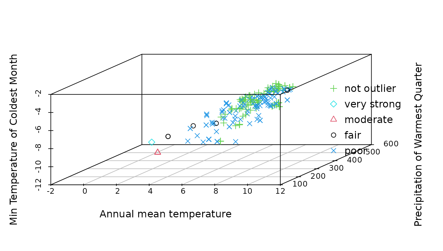

References

Amatulli, Giuseppe, et al. “Hydrography90m: A new high-resolution global hydrographic dataset.” Earth System Science Data 14.10 (2022): 4525-4550.
Harvey-Brown, Y., Barstow, M., Mark, J. & Rivers, M.C. 2017. Populus nigra. The IUCN Red List of Threatened Species 2017: e.T63530A68106816. https://dx.doi.org/10.2305/IUCN.UK.2017-3.RLTS.T63530A68106816.en. Accessed on 24 June 2024.
de Rigo, D., Enescu, C.M., Houston Durrant, T. and Caudullo, G. 2016. Populus nigra in Europe: distribution, habitat, usage and threats. European Atlas of Forest Tree Species, Publications Office of the European Union, Luxembourg.
Barstow, M. & Beech, E. 2018. Fagus sylvatica. The IUCN Red List of Threatened Species 2018: e.T62004722A62004725. https://dx.doi.org/10.2305/IUCN.UK.2018-1.RLTS.T62004722A62004725.en. Accessed on 24 June 2024.